fftl.transforms.sph_hankel

fftl.transforms.sph_hankel(mu, r, ar, *args, **kwargs)

Hankel transform with spherical Bessel functions

The spherical Hankel transform is here defined as

\[\tilde{a}(k) = \int_{0}^{\infty} \! a(r) \, j_\mu(kr) \, r^2 \, dr \;,\]

where \(j_\mu\) is the spherical Bessel function of order \(\mu\). The order can in general be any real or complex number. The transform is orthogonal, but unnormalised: applied twice, the original function is multiplied by \(\pi/2\).

Common special cases are \(\mu = 0\), which is related to the Fourier sine transform,

\[\tilde{a}(k) = \int_{0}^{\infty} \! a(r) \, \frac{\sin(kr)}{kr} \, r^2 \, dr \;,\]

and \(\mu = -1\), which is related to the Fourier cosine transform,

\[\tilde{a}(k) = \int_{0}^{\infty} \! a(r) \, \frac{\cos(kr)}{kr} \, r^2 \, dr \;.\]

Internally, the transform is computed as

\[\tilde{a}(k) = k^{\frac{\mu}{2}} \int_{0}^{\infty} \! \bigl[a(r) \, r^{2+\frac{\mu}{2}}\bigr] \, \bigl[(kr)^{-\frac{\mu}{2}} \, j_\mu(kr)\bigr] \, dr \;,\]

which is well-defined if \(|q| < 1 + \mathrm{Re} \, \frac{\mu}{2}\), where \(q\) is the bias parameter of the fftl() transform.

Examples

Compute the spherical Hankel transform for parameter mu = 1.

>>> # some test function
>>> x = 1/25
>>> r = np.logspace(-4, 2, 100)
>>> ar = 1/(r + x)**4
>>>
>>> # compute a biased transform
>>> from fftl.transforms import sph_hankel
>>> mu = 1.0
>>> k, ak = sph_hankel(mu, r, ar, q=0.22)

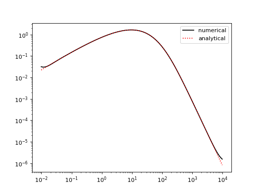
Compare with the analytical result.

>>> from scipy.special import sici
>>> si, ci = sici(k*x)
>>> u = np.pi*k*x*np.cos(k*x) + 2*np.pi*np.sin(k*x) - 2
>>> v = k*x*np.sin(k*x) - 2*np.cos(k*x)
>>> w = k*x*np.cos(k*x) + 2*np.sin(k*x)
>>> res = k*u/12 + k*ci*v/6 - k*si*w/6
>>>
>>> import matplotlib.pyplot as plt
>>> plt.loglog(k, ak, '-k', label='numerical')
>>> plt.loglog(k, res, ':r', label='analytical')
>>> plt.legend()
>>> plt.show()