Standard Integral Transforms
The fftl module provides Python implementations for a number of standard
integral transforms.
- class fftl.HankelTransform(mu: complex)
Hankel transform on a logarithmic grid.
The Hankel transform is here defined as
\[\tilde{a}(k) = \int_{0}^{\infty} \! a(r) \, J_\mu(kr) \, r \, dr \;,\]where \(J_\mu\) is the Bessel function of order \(\mu\). The order can in general be any real or complex number. The transform is orthogonal and normalised: applied twice, the original function is returned.
The Hankel transform is equivalent to a normalised spherical Hankel transform (
sph_hankel()) with the order and bias shifted by one half. Special cases are \(\mu = 1/2\), which is related to the Fourier sine transform,\[\tilde{a}(k) = \sqrt{\frac{2}{\pi}} \int_{0}^{\infty} \! a(r) \, \frac{\sin(kr)}{\sqrt{kr}} \, r \, dr \;,\]and \(\mu = -1/2\), which is related to the Fourier cosine transform,
\[\tilde{a}(k) = \sqrt{\frac{2}{\pi}} \int_{0}^{\infty} \! a(r) \, \frac{\cos(kr)}{\sqrt{kr}} \, r \, dr \;.\]Examples
Compute the Hankel transform for parameter
mu = 1.>>> import numpy as np >>> >>> # some test function >>> p, q = 2.0, 0.5 >>> r = np.logspace(-2, 2, 1000) >>> ar = r**p*np.exp(-q*r) >>> >>> # compute a biased transform >>> import fftl >>> hankel = fftl.HankelTransform(1.0) >>> k, ak = hankel(r, ar, q=0.1)
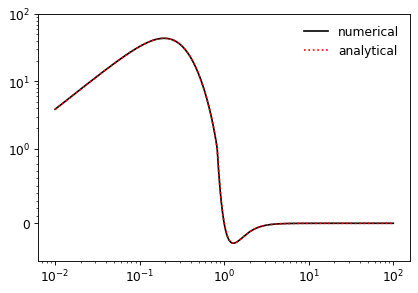
Compare with the analytical result.
>>> from scipy.special import gamma, hyp2f1
>>> res = k*q**(-3-p)*gamma(3+p)*hyp2f1((3+p)/2, (4+p)/2, 2, -(k/q)**2)/2
>>>
>>> import matplotlib.pyplot as plt
>>> plt.plot(k, ak, '-k', label='numerical')
>>> plt.plot(k, res, ':r', label='analytical')
>>> plt.xscale('log')
>>> plt.yscale('symlog', linthresh=1e0,
...            subs=np.arange(0.1, 1.0, 0.1))
>>> plt.ylim(-5e-1, 1e2)
>>> plt.legend()
>>> plt.show()
- class fftl.LaplaceTransform
Laplace transform on a logarithmic grid.
The Laplace transform is defined as
\[\tilde{a}(k) = \int_{0}^{\infty} \! a(r) \, e^{-kr} \, dr \;.\]Examples
Compute the Laplace transform using JAX.
>>> import jax.numpy as jnp
>>>
>>> # some test function
>>> p, q = 2.0, 0.5
>>> r = jnp.logspace(-2, 2, 1000)
>>> ar = r**p*jnp.exp(-q*r)
>>>
>>> # compute a biased transform
>>> import fftl
>>> laplace = fftl.LaplaceTransform()
>>> k, ak = laplace(r, ar, q=0.7)
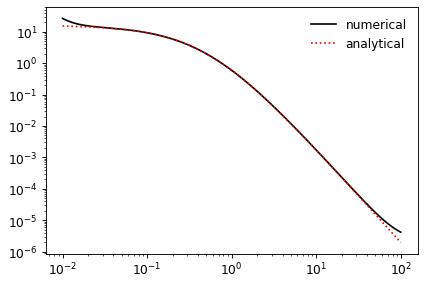
Compare with the analytical result.
>>> from jax.scipy.special import gamma
>>> res = gamma(p+1)/(q + k)**(p+1)
>>>
>>> import matplotlib.pyplot as plt
>>> plt.loglog(k, ak, '-k', label='numerical')
>>> plt.loglog(k, res, ':r', label='analytical')
>>> plt.legend()
>>> plt.show()
- class fftl.SphericalHankelTransform(mu: complex)
Hankel transform with spherical Bessel functions.
The spherical Hankel transform is here defined as
\[\tilde{a}(k) = \int_{0}^{\infty} \! a(r) \, j_\mu(kr) \, r^2 \, dr \;,\]where \(j_\mu\) is the spherical Bessel function of order \(\mu\). The order can in general be any real or complex number. The transform is orthogonal, but unnormalised: applied twice, the original function is multiplied by \(\pi/2\).
The spherical Hankel transform is equivalent to an unnormalised Hankel transform (
hankel()) with the order and bias shifted by one half. Special cases are \(\mu = 0\), which is related to the Fourier sine transform,\[\tilde{a}(k) = \int_{0}^{\infty} \! a(r) \, \frac{\sin(kr)}{kr} \, r^2 \, dr \;,\]and \(\mu = -1\), which is related to the Fourier cosine transform,
\[\tilde{a}(k) = \int_{0}^{\infty} \! a(r) \, \frac{\cos(kr)}{kr} \, r^2 \, dr \;.\]Examples
Compute the spherical Hankel transform for parameter
mu = 1.>>> import numpy as np >>> >>> # some test function >>> p, q = 2.0, 0.5 >>> r = np.logspace(-2, 2, 1000) >>> ar = r**p*np.exp(-q*r) >>> >>> # compute a biased transform >>> import fftl >>> sph_hankel = fftl.SphericalHankelTransform(1.0) >>> k, ak = sph_hankel(r, ar, q=0.1)
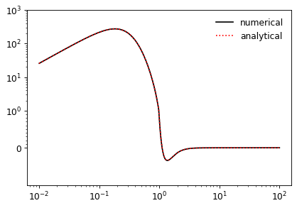
Compare with the analytical result.
>>> from scipy.special import gamma
>>> u = (1 + k**2/q**2)**(-p/2)*q**(-p)*gamma(1+p)/(k**2*(k**2 + q**2)**2)
>>> v = k*(k**2*(2 + p) - p*q**2)*np.cos(p*np.arctan(k/q))
>>> w = q*(k**2*(3 + 2*p) + q**2)*np.sin(p*np.arctan(k/q))
>>> res = u*(v + w)
>>>
>>> import matplotlib.pyplot as plt
>>> plt.plot(k, ak, '-k', label='numerical')
>>> plt.plot(k, res, ':r', label='analytical')
>>> plt.xscale('log')
>>> plt.yscale('symlog', linthresh=1e0,
...            subs=np.arange(0.1, 1.0, 0.1))
>>> plt.ylim(-1e0, 1e3)
>>> plt.legend()
>>> plt.show()
- class fftl.StieltjesTransform(rho: float)
Generalised Stieltjes transform on a logarithmic grid.
The generalised Stieltjes transform is defined as
\[\tilde{a}(k) = \int_{0}^{\infty} \! \frac{a(r)}{(k + r)^\rho} \, dr \;,\]where \(\rho\) is a positive real number.
The integral can be computed as a
fftl()transform in \(k' = k^{-1}\) if it is rewritten in the form\[\tilde{a}(k) = k^{-\rho} \int_{0}^{\infty} \! a(r) \, \frac{1}{(1 + k'r)^\rho} \, dr \;.\]Warning
The Stieltjes FFTLog transform is often numerically difficult.
Examples
Compute the generalised Stieltjes transform with
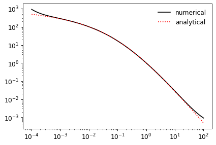
rho = 2.>>> import numpy as np >>> >>> # some test function >>> s = 0.1 >>> r = np.logspace(-4, 2, 100) >>> ar = r/(s + r)**2 >>> >>> # compute a biased transform with shift >>> import fftl >>> stieltjes = fftl.StieltjesTransform(2.) >>> k, ak = stieltjes(r, ar, kr=1e-2)
Compare with the analytical result.
>>> res = (2*(s-k) + (k+s)*np.log(k/s))/(k-s)**3
>>>
>>> import matplotlib.pyplot as plt
>>> plt.loglog(k, ak, '-k', label='numerical')
>>> plt.loglog(k, res, ':r', label='analytical')
>>> plt.legend()
>>> plt.show()
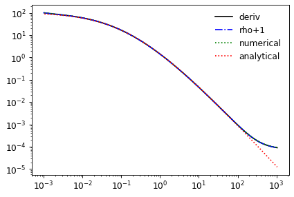
Compute the derivative in two ways and compare with numerical and analytical results.
>>> # compute Stieltjes transform with derivative
>>> k, ak, akp = stieltjes(r, ar, kr=1e-1, deriv=True)
>>>
>>> # derivative by rho+1 transform
>>> stieltjes_d = fftl.StieltjesTransform(stieltjes.rho+1)
>>> k_, takp = stieltjes_d(r, ar, kr=1e-1)
>>> takp *= -stieltjes.rho*k_
>>>
>>> # numerical derivative
>>> nakp = np.gradient(ak, np.log(k))
>>>
>>> # analytical derivative
>>> aakp = -((-5*k**2+4*k*s+s**2+2*k*(k+2*s)*np.log(k/s))/(k-s)**4)
>>>
>>> # show
>>> plt.loglog(k, -akp, '-k', label='deriv')
>>> plt.loglog(k_, -takp, '-.b', label='rho+1')
>>> plt.loglog(k, -nakp, ':g', label='numerical')
>>> plt.loglog(k, -aakp, ':r', label='analytical')
>>> plt.legend()
>>> plt.show()