Generalised FFTLog¶

The functionality of the fftl module is provided by the fftl.transform() routine to compute the generalised FFTLog integral transform for a given kernel.

fftl.transform(u, r, ar, *, q=0.0, kr=1.0, low_ringing=True, deriv=False)¶

Generalised FFTLog for integral transforms.

Computes integral transforms for arbitrary kernels using a generalisation of Hamilton’s method [1] for the FFTLog algorithm [2].

The kernel of the integral transform is characterised by the coefficient function u, see notes below, which must be callable and accept complex input arrays.

The function to be transformed must be given on a logarithmic grid r. The result of the integral transform is similarly computed on a logarithmic grid k = kr/r, where kr is a scalar constant (default: 1) which shifts the logarithmic output grid. The selected value of kr is automatically changed to the nearest low-ringing value if low_ringing is true (the default).

The integral transform can optionally be biased, see notes below.

The function can optionally at the same time return the derivative of the integral transform with respect to the logarithm of k, by setting deriv to true.

Parameters:

ucallable: Coefficient function. Must have signature u(x) and support complex input arrays.
rarray_like (N,): Grid of input points. Must have logarithmic spacing.
ararray_like (…, N): Function values. If multidimensional, the integral transform applies to the last axis, which must agree with input grid.
qfloat, optional: Bias parameter for integral transform.
krfloat, optional: Shift parameter for logarithmic output grid.
low_ringingbool, optional: Change given kr to the nearest value fulfilling the low-ringing condition.
derivbool, optional: Also return the first derivative of the integral transform.

Returns:

karray_like (N,): Grid of output points.
akarray_like (…, N): Integral transform evaluated at k.
dakarray_like (…, N), optional: If deriv is true, the derivative of ak with respect to the logarithm of k.

Notes

Computes integral transforms of the form

\[\tilde{a}(k) = \int_{0}^{\infty} \! a(r) \, T(kr) \, dr\]

for arbitrary kernels \(T\).

If \(a(r)\) is given on a logarithmic grid of \(r\) values, the integral transform can be computed for a logarithmic grid of \(k\) values with a modification of Hamilton’s FFTLog algorithm,

\[U(x) = \int_{0}^{\infty} \! t^x \, T(t) \, dt \;.\]

The generalised FFTLog algorithm therefore only requires the coefficient function \(U\) for the given kernel. Everything else, and in particular how to construct a well-defined transform, remains exactly the same as in Hamilton’s original algorithm.

The transform can optionally be biased,

\[\tilde{a}(k) = k^{-q} \int_{0}^{\infty} \! [a(r) \, r^{-q}] \, [T(kr) \, (kr)^q] \, dr \;,\]

where \(q\) is the bias parameter. The respective biasing factors \(r^{-q}\) and \(k^{-q}\) for the input and output values are applied internally.

References

[1]

Hamilton A. J. S., 2000, MNRAS, 312, 257 (astro-ph/9905191)

[2]

Talman J. D., 1978, J. Comp. Phys., 29, 35

Examples

Compute the one-sided Laplace transform of the hyperbolic tangent function. The kernel of the Laplace transform is \(\exp(-kt)\), which determines the coefficient function.

>>> import numpy as np
>>> from scipy.special import gamma, digamma
>>>
>>> def u_laplace(x):
...     # requires Re(x) = q > -1
...     return gamma(1 + x)

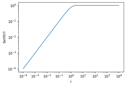
Create the input function values on a logarithmic grid.

>>> r = np.logspace(-4, 4, 100)
>>> ar = np.tanh(r)
>>>
>>> import matplotlib.pyplot as plt
>>> plt.loglog(r, ar)
>>> plt.xlabel('$r$')
>>> plt.ylabel('$\\tanh(r)$')
>>> plt.show()

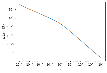
Compute the Laplace transform, and compare with the analytical result.

>>> import fftl
>>> k, ak = fftl.transform(u_laplace, r, ar)
>>>
>>> lt = (digamma((k+2)/4) - digamma(k/4) - 2/k)/2
>>>
>>> plt.loglog(k, ak)
>>> plt.loglog(k, lt, ':')
>>> plt.xlabel('$k$')
>>> plt.ylabel('$L[\\tanh](k)$')
>>> plt.show()

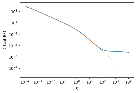
The numerical Laplace transform has an issue on the right, which is due to the circular nature of the FFTLog integral transform. The effect is mitigated by computing a biased transform with q = 0.5. Good values of the bias parameter q depend on the shape of the input function.

>>> k, ak = fftl.transform(u_laplace, r, ar, q=0.5)
>>>
>>> plt.loglog(k, ak)
>>> plt.loglog(k, lt, ':')
>>> plt.xlabel('$k$')
>>> plt.ylabel('$L[\\tanh](k)$')
>>> plt.show()