fftl.transforms.sph_hankel

fftl.transforms.sph_hankel(mu, r, ar, *args, **kwargs)

Hankel transform with spherical Bessel functions

The spherical Hankel transform is here defined as

\[\tilde{a}(k) = \int_{0}^{\infty} \! a(r) \, j_\mu(kr) \, r^2 \, dr \;,\]

where \(j_\mu\) is the spherical Bessel function of order \(\mu\). The order can in general be any real or complex number. The transform is orthogonal, but unnormalised: applied twice, the original function is multiplied by \(\pi/2\).

The spherical Hankel transform is equivalent to an unnormalised Hankel transform (hankel()) with the order and bias shifted by one half. Special cases are \(\mu = 0\), which is related to the Fourier sine transform,

\[\tilde{a}(k) = \int_{0}^{\infty} \! a(r) \, \frac{\sin(kr)}{kr} \, r^2 \, dr \;,\]

and \(\mu = -1\), which is related to the Fourier cosine transform,

\[\tilde{a}(k) = \int_{0}^{\infty} \! a(r) \, \frac{\cos(kr)}{kr} \, r^2 \, dr \;.\]

Examples

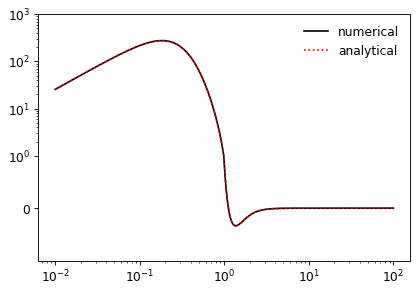
Compute the spherical Hankel transform for parameter mu = 1.

>>> # some test function
>>> p, q = 2.0, 0.5
>>> r = np.logspace(-2, 2, 1000)
>>> ar = r**p*np.exp(-q*r)
>>>
>>> # compute a biased transform
>>> from fftl.transforms import sph_hankel
>>> mu = 1.0
>>> k, ak = sph_hankel(mu, r, ar, q=0.1)

Compare with the analytical result.

>>> from scipy.special import gamma
>>> u = (1 + k**2/q**2)**(-p/2)*q**(-p)*gamma(1+p)/(k**2*(k**2 + q**2)**2)
>>> v = k*(k**2*(2 + p) - p*q**2)*np.cos(p*np.arctan(k/q))
>>> w = q*(k**2*(3 + 2*p) + q**2)*np.sin(p*np.arctan(k/q))
>>> res = u*(v + w)
>>>
>>> import matplotlib.pyplot as plt
>>> plt.plot(k, ak, '-k', label='numerical')
>>> plt.plot(k, res, ':r', label='analytical')
>>> plt.xscale('log')
>>> plt.yscale('symlog', linthresh=1e0, subs=[2, 3, 4, 5, 6, 7, 8, 9])
>>> plt.ylim(-1e0, 1e3)
>>> plt.legend()
>>> plt.show()