fftl.transforms.stieltjes

fftl.transforms.stieltjes(rho, r, ar, q=0.0, kr=1.0, **kwargs)

Generalised Stieltjes transform

The generalised Stieltjes transform is defined as

\[\tilde{a}(k) = \int_{0}^{\infty} \! \frac{a(r)}{(k + r)^\rho} \, dr \;,\]

where \(\rho\) is a positive real number.

The integral can be computed as a fftl() transform in \(k' = k^{-1}\) if it is rewritten in the form

\[\tilde{a}(k) = k^{-\rho} \int_{0}^{\infty} \! a(r) \, \frac{1}{(1 + k'r)^\rho} \, dr \;.\]

Warning

The Stieltjes FFTLog transform is often numerically difficult.

Examples

Compute the generalised Stieltjes transform with rho = 2.

>>> # some test function
>>> s = 0.1
>>> r = np.logspace(-4, 2, 100)
>>> ar = r/(s + r)**2
>>>
>>> # compute a biased transform with shift
>>> from fftl.transforms import stieltjes
>>> rho = 2.
>>> k, ak = stieltjes(rho, r, ar, q=-0.2, kr=1e-2)

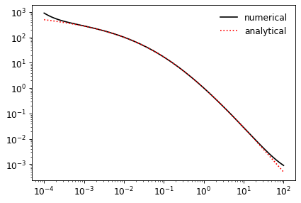
Compare with the analytical result.

>>> res = (2*(s-k) + (k+s)*np.log(k/s))/(k-s)**3
>>>
>>> import matplotlib.pyplot as plt
>>> plt.loglog(k, ak, '-k', label='numerical')
>>> plt.loglog(k, res, ':r', label='analytical')
>>> plt.legend()
>>> plt.show()

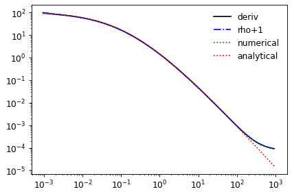
Compute the derivative in two ways and compare with numerical and analytical results.

>>> # compute Stieltjes transform with derivative
>>> k, ak, akp = stieltjes(rho, r, ar, kr=1e-1, deriv=True)
>>>
>>> # derivative by rho+1 transform
>>> k_, takp = stieltjes(rho+1, r, ar, kr=1e-1)
>>> takp *= -rho*k_
>>>
>>> # numerical derivative
>>> nakp = np.gradient(ak, np.log(k))
>>>
>>> # analytical derivative
>>> aakp = -((-5*k**2+4*k*s+s**2+2*k*(k+2*s)*np.log(k/s))/(k-s)**4)
>>>
>>> # show
>>> plt.loglog(k, -akp, '-k', label='deriv')
>>> plt.loglog(k_, -takp, '-.b', label='rho+1')
>>> plt.loglog(k, -nakp, ':g', label='numerical')
>>> plt.loglog(k, -aakp, ':r', label='analytical')
>>> plt.legend()
>>> plt.show()